Microfacet BRDFs from Scratch

In this article, I will derive these famous Specular and Diffuse BRDFs from scratch.

$\boxed{\text{BRDF}_{\text{spec}} = \frac{F(\omega_i, \omega_h)\, G_1(\omega_i, \omega_o, \omega_h)\, D(\omega_h)}{4\,|\omega_g \cdot \omega_i|\,|\omega_g \cdot \omega_o|}}$

$\text{BRDF}_{\text{diff}} = \frac{1}{|\omega_g \cdot \omega_i|\,|\omega_g \cdot \omega_o|} \int_\Omega \frac{1}{\pi}\, \langle \omega_i \cdot \omega_m \rangle\, G_1(\omega_i, \omega_o, \omega_m)\, D(\omega_m)\, \langle \omega_o \cdot \omega_m \rangle\, d\omega_m$

I will try to make the derivations as intuitive as possible with figures and explanations. The interactive HTML sections have been written by AI (The free version of Claude) as I don't know how to do frontend HTML programming. The other figures were made by me using inkscape.

This derivation is not novel, I read through 5 very important papers shuffling all of them at once, and I got the idea while going through them, to create a straight-forward article for someone like me, who is interested in mathematics and derivations of equations, but for whom, certain jumps in derivations don't come so naturally.

Contents

1. Important Symbols
2. The BRDF
3. Microgeometry and Microfacets
4. Visible Microfacets
5. Statistical BRDFs
6. Specular BRDF
7. Diffuse BRDF
8. Deriving the Diffuse Micro-BRDF
9. Conclusion
10. References

Important Symbols

Symbol	Meaning
$L_o$	Outgoing radiance
$E_i$	Irradiance
$L_i$	Incoming radiance
$\omega_g$	Macrosurface normal
$\omega_o$	Outgoing direction (w.r.t. surface normal)
$\omega_i$	Incoming direction (w.r.t. surface normal)
$\theta_i$	Elevation angle - angle w.r.t. the polar axis of the sphere
$\phi_i$	Azimuth angle - angle w.r.t. the equatorial plane of the sphere
$\omega_h$	Half-vector: $\widehat{\omega_o + \omega_i}$
$d\omega$	Differential solid angle
$D(\omega_m)$	Normal Distribution Function (NDF)
$G_1$	Masking-shadowing function
$F$	Fresnel factor
$\langle \omega_i \cdot \omega_m \rangle$	Clamped dot product.

The BRDF

When a light hits any "thing", it will either be transmitted (refracted), reflected, or absorbed. Absorption happens when the atom that is hit by the light takes the energy of the light and it reaches an excited state. Eventually, the energy is spit out, if it's emitted as visible light then that phenomenon is known as Photoluminescence. This isn't really important to Rendering as we rarely have to simulate that phenomena on production or real-time renderers. BRDF deals with the reflection of light. If we want to emulate the transmission as well, it'll require another function with a very similar name, the BTDF.

Bi-directional Reflectance Distribution Function (BRDF) is a scary name, but it is quite simple. It gets a bad reputation because when people try to learn it, they get met with very scary looking equations (some of which we will derive in this article).

The BRDF is simply the ratio of outgoing radiance in a given direction to the differential irradiance from a specific incoming direction. Radiance is the power of light in a point in a single direction. Irradiance is the power of light in a point from all directions. That is why we use differential irradiance. If we take an integral of the differential irradiance, we get the whole irradiance. I came across this cheatsheet in the graphics programming discord for important terms in rendering such as radiance, irradiance and what not.

So, BRDF $= L_o / E_i$ then? Yes! But, we don't actually know the $E_i$ in rendering. We will have to figure out the Irradiance by taking the incoming light from each angle around the point and integrating it. Taking the irradiance of each angle is not practical at all, there's infinite angles as there are infinite numbers. So we use something called a differential solid angle, which is an infinitesmally small surface 'patch' in a sphere. As that patch is extremely small, the irradiance along the surface at any point will be virtually the same, so we can measure the irradiance at one point in the surface and then project that patch to the point.

The surface area of the patch, despite being extremely small, is larger than that of a singular 'point' of whose BRDF we are measuring. Depending on the angle at which the patch is located with respect to the normal, the incoming light gets spread out and misses the point.

Figure 1. Interactive visualiser showing how the same solid angle $d\omega$ projects onto a larger surface element $dA$ as the incident angle $\theta$ increases.

Due to this, the incoming light at a point through a solid angle will then become:

$L_i \cos\theta_i \, d\omega_i$

(irradiance through dω)

$L_i$ is the incoming light from a direction $i$, $\theta_i$ is the light incident angle wrt normal, and $d\omega$ is the differentiable solid angle.

So the BRDF is:

$\text{BRDF} = \frac{L_o}{L_i \cos\theta_i \, d\omega_i}$

In rendering, we mostly want to figure out the Radiance to a specific directions, so we write it as:

$$\text{BRDF} = \frac{dL_o}{L_i \cos\theta_i \, d\omega_i} \tag{i}$$

BRDFs have two physical properties:

Conservation of energy — the total reflected energy cannot exceed the incident energy:

$\int_\Omega f_r \cos\theta_o \, d\omega_o \leq 1$

Reciprocity — swapping incoming and outgoing directions leaves the BRDF unchanged:

$f_r(\theta_i, \phi_i, \theta_o, \phi_o) = f_r(\theta_o, \phi_o, \theta_i, \phi_i)$

Microgeometry and Microfacets

A 'smooth' surface to our eye will have extreme difference in elevation as we zoom in. There will be many bumps in the microscopic scale.

Figure 2. A macrosurface that appears smooth has microsurfaces with varying normals at the microscopic scale.

If we want a realistic simulation of light then we cannot ignore this scale. We are not going to nanogeometry however, we will only think of any surface as being built up of very small microsurfaces. Each point we want to sample on the macrosurface (which may appear as a pixel on our screen) will have microsurfaces. So if we want to figure out the total radiated light in a certain direction for a certain point in the macrosurface, we need to find the radiation for that direction throughout all the points in the microsurface and sum all of it. Since these microsurfaces are very small, the out-radiance angle for each point of the microsurface will be parallel to one-another. This can be visualised as each point projecting itself to a straight line.

Figure 3. The microsurface points all project onto a line of width $\cos\theta_{\omega_o}$ in the outgoing direction $\omega_o$.

The area of the projection will be:

$$\text{ProjArea} = 1 \cdot \cos(\theta_{\omega_o}) \tag{ii}$$

The points in the microsurface will have different normals so each point's out-radiance will be spread out in the outgoing direction. If the normal of a point in the microsurface is parallel to the outgoing direction, the out-radiance will be projected 1:1 to the projected 'line', while for any other angle the out-radiance will be spread out.

Let $\mathcal{M}$ be the Micro-geometry.

$$L(\omega_o, \mathcal{M}) = \frac{\displaystyle\int_\mathcal{M} \text{projArea}(p_m)\, L(\omega_o, p_m)\, dp_m}{\displaystyle\int_\mathcal{M} \text{projArea}(p_m)\, dp_m} \tag{iii}$$

This formula acts as a weighted average of the out-radiance of each point of the microsurface. An intuitive metaphor is to imagine a folding phone, if it's folded 90 degrees and you're looking at it. The folded screen that is directly facing your eyes will contribute more to the brightness than the one that is facing up, and is 90 degrees to your eyes.

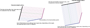
Figure 4. The folding phone analogy: the screen directly facing the viewer contributes more brightness than the one at 90 degrees. Each microsurface point contributes proportionally to its projected area.

For a macrosurface with microsurfaces, let us create a function $D(\omega)$ which counts the amount of points in the microsurface with a specific normal $\omega$.

$$D(\omega) = \int_\mathcal{M} \delta_\omega\!\left(\omega_m(p_m)\right) dp_m \tag{iv}$$

$\delta_\omega$ is known as a dirac delta, think of it as a function that discards what is not expected. $\delta_\omega$ means that the delta will discard every input which isn't $\omega$. $\omega_m(p_m)$ gives the normal of the microsurface point $p_m$. So, $D(\omega)$ gives the total points in the microsurface with the given normal $\omega$.

There's an infinite amount of vectors as normals that a point can have. These normals exist in a unit sphere as well. A unit sphere also has all the normals in 3-D. For each point in the microsurface with a normal $\omega_m$, there's a point in the unit sphere with that normal. For a subset of point in the microsurface $\mathcal{M}' \subseteq \mathcal{M}$, there is a subset of unit sphere $\Omega' \subseteq \Omega$ with the same normals.

$$\int_{\mathcal{M}'} dp_m = \int_{\Omega'} D(\omega_m)\, d\omega_m \tag{area}$$

Integrating for each point in $\mathcal{M}'$ gives the same 'area' as integrating for each point in a unit sphere with the same normals, because $D(\omega_m)$ gives the weight for each of those normals. Reminder that even in the unit sphere integral, the $D(\omega_m)$ goes through each point in the microsurface and checks the normal of each point. So, for the whole microsurface, or the whole unit circle, it gives the microsurface area.

Visible microfacets

Since a surface is made up of microsurfaces (Figure 2), the projections will be that of each point in the microsurfaces. Not all the points in the microsurfaces are actually visible, depending on the viewing angle. The visibility also depends on what's known as a 'microsurface profile'. The same distribution of normals can have different behaviors and have different visibility depending on how the normals are distributed along the microsurfaces.

Figure 5. Two microsurfaces with the same normal distribution but different profiles can have different visibility. Some points are occluded depending on the viewing direction $\omega_o$.

The projected area of the microsurfaces can be viewed as such:

$$\text{ProjArea}_\mathcal{M} = \int_\mathcal{M} G(\omega_o, p_m)\, \langle \omega_o \cdot \omega_m(p_m) \rangle \, dp_m$$

$G$ here is a function that evaluates to 0 if a point $p_m$ is blocked, and 1 if it's not blocked. Clamp function is used to cull out backfacing microgeometries, as it'll clamp negative value to 0, so if there's a point which faces the opposite of $\omega_o$, it'll not contribute to the projected area. We can create another $G$ function that takes $\omega_m$ instead of $p_m$ [2]. For that:

$$\text{ProjArea}_\mathcal{M} = \int_\Omega G_1(\omega_o, \omega_m)\, \langle \omega_o \cdot \omega_m \rangle\, D(\omega_m)\, d\omega_m \tag{v}$$

Here, $D(\omega_m)$ gives weight to the specific $\omega_m$. Meaning, if there's more points with a specific $\omega_m$ which are also visible, their contribution has more weight. Since the projected area is the area of all visible points in the microsurface, for a surface of unit area, we know that its area from (ii). From (ii) and (v) we get:

$$\cos(\theta_{\omega_o}) = \int_\Omega G_1(\omega_o, \omega_m)\, \langle \omega_o \cdot \omega_m \rangle\, D(\omega_m)\, d\omega_m \tag{vi}$$

In equation (iii), let us replace the denominator with (ii). We can replace the whole integral in the numerator with another numerator that also takes the area (v), and for the function $L(\omega_o, p_m)$, which is a function of the point, we can just convert it to a function of $\omega_m$: $L(\omega_o, \omega_m)$. (The reason it's so easy to convert is because the radiance depends on the normal of the point regardless).

$$L(\omega_o, \mathcal{M}) = \frac{\displaystyle\int_\Omega L(\omega_o, \omega_m)\, G_1(\omega_o, \omega_m)\, D(\omega_m)\, \langle \omega_o \cdot \omega_m \rangle \, d\omega_m}{\cos(\theta_{\omega_o})} \tag{vii}$$ $$L(\omega_o, \mathcal{M}) = \int_\Omega L(\omega_o, \omega_m)\, D_{\omega_o}(\omega_m)\, d\omega_m \tag{viii}$$

Here, $D_{\omega_o}(\omega_m)$ acts as a distribution of the visible normals, it gives value between 0 and 1.

$$D_{\omega_o}(\omega_m) = \frac{G_1(\omega_o, \omega_m)\, D(\omega_m)\, \langle \omega_o \cdot \omega_m \rangle}{\cos(\theta_{\omega_o})} \tag{ix}$$

Statistical BRDFs

$L(\omega_o, \omega_m)$ is the outgoing radiance at a direction $\omega_m$. Using basic calculus, we can rewrite it as:

$$L(\omega_o, \omega_m) = \int_{\Omega_i} \frac{dL(\omega_o, \omega_m)}{d\omega_i}\, d\omega_i \tag{x}$$

Basically, we differentiate the function wrt $d\omega_i$ and integrate it along $d\omega_i$. From (i), we can say that the micro BRDF, $\text{BRDF}_m$ (It is a function of $\omega_o$, $\omega_i$, and $\omega_m$) for a specific microsurface is:

$$\text{BRDF}_m = \frac{dL_o}{L(\omega_i)\, \langle \omega_i \cdot \omega_m \rangle\, d\omega_i}$$

We can ignore the back faces using the clamp, so:

$$\frac{dL_o}{d\omega_i} = \text{BRDF}_m \cdot L(\omega_i) \cdot \langle \omega_i \cdot \omega_m \rangle \tag{xi}$$

Substituting (xi) into (x):

$$L(\omega_o, \omega_m) = \int_{\Omega_i} L(\omega_i)\, \text{BRDF}_m\, \langle \omega_i \cdot \omega_m \rangle\, d\omega_i \tag{xiii}$$

Now, let's differentiate equation (viii) with respect to the incoming irradiance:

$$dL(\omega_o, \mathcal{M}) = \int_\Omega dL(\omega_o, \omega_m)\, G_1(\omega_o, \omega_m)\, D_{\omega_o}(\omega_m)\, d\omega_m \tag{xiv}$$

We replace $dL_o$ from (xi) in (xiv):

$$dL(\omega_o, \mathcal{M}) = L(\omega_i)\, d\omega_i \int_\Omega \text{BRDF}_m\, \langle \omega_i \cdot \omega_m \rangle\, G_1(\omega_o, \omega_m)\, D_{\omega_o}(\omega_m)\, d\omega_m \tag{xv}$$

The macro BRDF is given in (i). We can replace the $dL_o$ with (xv), then replace $D_{\omega_o}(\omega_m)$ from (ix). $\cos(\theta_{\omega_o})$ and $\cos(\theta_i)$ can be taken out of the integral and written as $|\omega_g \cdot \omega_i|$ and $|\omega_g \cdot \omega_o|$ as they depend on the macro surface normal:

$$\text{BRDF} = \frac{1}{|\omega_g \cdot \omega_i|\,|\omega_g \cdot \omega_o|} \int_\Omega \text{BRDF}_m\, \langle \omega_i \cdot \omega_m \rangle\, G_1(\omega_i, \omega_o, \omega_m)\, D(\omega_m)\, \langle \omega_o \cdot \omega_m \rangle\, d\omega_m \tag{xvi}$$

This statistical model of BRDF covers the light before it bounces from the microsurface. After it bounces, it could get blocked by another microsurface, for that, we use a function known as the shadow-masking function ($G_1$). It will take into account the incident direction of the light as well. This is the general form of a BRDF. If we assume the microfacets to be a perfect mirror then we will get Specular BRDF and if we assume it to be a perfect lambertian surface that diffsue light, then we get the Diffuse BRDF.

Specular BRDF

A simple generic specular BSDF will look like this [3]:

$$f_s = \rho \cdot \frac{\delta_{\omega_s}(\omega_o)}{|\omega_o \cdot \omega_m|} \tag{xvii}$$

$\rho$ is the fraction of out-radiance. $\omega_s$ is the angle of specular reflection. $|\omega_o \cdot \omega_m|$ is there to cancel out the $|\omega_o \cdot \omega_m|$ numerator in the macro surface BSDF integral.

If we assume only a specular reflection then for a given $\omega_i$ and $\omega_o$, there is at most only 1 $\omega_m$ that scatters the energy from $\omega_i$ to $\omega_o$ directly. That normal is $\omega_h$ and $\omega_m$ (also known as the half vector): $\omega_h = \omega_i + \omega_o$.

In this case, we can re-write $f_s$ in terms of $\omega_h$:

$$f_s = \rho \cdot \frac{\delta_{\omega_h}(\omega_m)}{|\omega_o \cdot \omega_m|} \cdot \left\|\frac{d\omega_h}{d\omega_o}\right\| \tag{xviii}$$

The $\delta_{\omega_s}(\omega_o)$ is just a shorthand for writing $\int \delta(\omega_o - \omega_s)\, d\omega_o$. We want the equation (xvii) in the form of $\omega_h$ and $\omega_m$ instead. The delta will be changed to $\delta_{\omega_h}(\omega_m)$. The dirac delta always has an associated element [3]. The dirac delta in (xvii) has $d\omega_o$ associated with itself. When changing it to be associated with $d\omega_h$, we need to find the jacobian so that it scales properly.

The jacobian must be $\|d\omega_m/d\omega_o\| = \|d\omega_m/d\omega_h \cdot d\omega_h/d\omega_o\|$. Since the delta function means that only those $\omega_m$ that are $\omega_h$ are considered, we can say that $d\omega_m/d\omega_h = 1$. So, $\|d\omega_m/d\omega_o\| = \|d\omega_h/d\omega_o\|$.

The jacobian can be written as:

$$\frac{d\omega_h}{d\omega_o} = \frac{|\omega_o \cdot \omega_h|}{\|\tilde{h}\|^2} \tag{xix}$$

This gives the ratio of how much a change in solid angle of $d\omega_o$ corresponds to a change in the solid angle of $d\omega_h$. We will see that the size of the solid angle patch $d\omega_h$ depends on the length of the $\tilde{h}$ vector.

Figure 6. Interactive Jacobian visualiser. Drag the i (red) and o (green) arrowheads or use the sliders. The green wedge $d\omega_o$ lives on the circle centred at the tip of $\mathbf{i}$; the dark wedge $d\omega_h$ lives on the central unit sphere. The dashed lines show the projection. Notice how $d\omega_h \ll d\omega_o$ when $\mathbf{i}$ and $\mathbf{o}$ are nearly parallel.

We know $\|\tilde{h}\| = \tilde{h} \cdot \hat{h}$. If we do a dot product of a vector with its unit self, we get its length, as $\theta = 0$, only the magnitude will remain. Putting this magnitude value in (xix):

$$\frac{d\omega_h}{d\omega_o} = \frac{|\omega_o \cdot \omega_h|}{(\tilde{h} \cdot \hat{h})^2} = \frac{|\omega_o \cdot \omega_h|}{((\omega_o + \omega_i) \cdot \hat{h})^2} = \frac{|\omega_o \cdot \omega_h|}{(\omega_o \cdot \hat{h} + \omega_i \cdot \hat{h})^2} = \frac{|\omega_o \cdot \omega_h|}{(2\,\omega_o \cdot \hat{h})^2} = \frac{1}{4|\omega_o \cdot \omega_h|} \tag{xx}$$

($\omega_o \cdot \hat{h} = \omega_i \cdot \hat{h}$ because $\hat{h}$ is a bisector of $\omega_o$ and $\omega_i$.)

Putting this value in (xviii):

$$f_s = \frac{F \cdot \delta_{\omega_h}(\omega_m)}{4\,|\omega_o \cdot \omega_m|\,|\omega_o \cdot \omega_h|} \tag{xxi}$$

For reflection, the fraction of out radiance is the Fresnel factor. Since $f_s$ is the micro brdf for specular reflections, We replace $\text{BRDF}_m$ with $f_s$ in (xvi). Due to the delta function, we can discard all the $\omega_m$s that are not $\omega_h$ and we can remove the integral. Cancelling the dot products:

$$\boxed{\text{BRDF}_{\text{spec}} = \frac{F(\omega_i, \omega_h)\, G_1(\omega_i, \omega_o, \omega_h)\, D(\omega_h)}{4\,|\omega_g \cdot \omega_i|\,|\omega_g \cdot \omega_o|}} \tag{xxii}$$

This is the Specular form of the macro BRDF. It can be solved by choosing appropriate $G_1$ and $D$ functions. Most of the engines in real time rendering use the GGX $D$ and $G_1$ functions.

Diffuse BRDFs

It is well known that the Diffuse micro BRDF $= 1/\pi$. So the diffuse BRDF will just be:

$$\text{BRDF}_{\text{diff}} = \frac{1}{|\omega_g \cdot \omega_i|\,|\omega_g \cdot \omega_o|} \int_\Omega \frac{1}{\pi}\, \langle \omega_i \cdot \omega_m \rangle\, G_1(\omega_i, \omega_o, \omega_m)\, D(\omega_m)\, \langle \omega_o \cdot \omega_m \rangle\, d\omega_m \tag{xxiii}$$

This equation is actually not solved by renderers. Either approximations are used or there's sampling done for a number of incoming light direction using monte carlo simulation.

Diffuse micro BRDF

Remember that a physically accurate BRDF has the property of conservation of energy:

$$\int_\Omega \text{BRDF} \cos\theta_o \, d\omega_o \leq 1$$

$d\omega$ is a surface element of a sphere, also known as a solid angle. $d\omega$ is very small, so it acts as a rectangle. The area of a rectangle is the width $\times$ length. If we are to find the area of $d\omega$, we only need the length and the width of the surface element.

We are used to dividing spheres into latitudes and longitudes. The longitudinal lines are great circles (the largest straight lines we can make on a sphere). The longitudinal lines extend from one pole to another. Two longitudinal lines will converge near the pole and separate the farthest at the equator. The horizontal lines are parallel to each other, they don't converge and two parallel lines are equally spaced out all around the circle.

$d\theta$ is the difference in angle between the top and bottom sides (the length).

Figure 7. The surface element $d\omega$ on a unit sphere. Its height is $d\theta$ and its width scales as $\sin\theta \, d\phi$, shrinking to zero at the poles.

The width of the surface element depends on where the surface element is. Depending on where the surface element is, the width may be $d\phi$ near the equator, or it may even reach 0 if the surface element is near the poles. We can scale the size by its elevation, if it's towards the pole (elevation increases), the width tends to 0. With elevation 0, the width becomes $d\phi$. This behavior can be modeled by the sine of the elevation angle. So we can say that the width $= \sin(\theta)\, d\phi$. The area then becomes:

$$d\omega = \sin\theta \, d\phi \, d\theta \tag{dω}$$

In this equation, we replace $d\omega_o$:

$$\int_\Omega \text{BRDF} \cos\theta_o \sin\theta_o \, d\phi_o \, d\theta_o \leq 1$$

Since we assume a perfect diffuse behavior, the diffuse reflection reflects the light in all direction equally. Solving the integral:

$$\int_0^{2\pi}\!\int_0^{\pi/2} \text{BRDF} \cos\theta_o \sin\theta_o \, d\theta_o \, d\phi_o = 1$$ $$\int_0^{2\pi} \text{BRDF} \left[\frac{\sin^2\theta_o}{2}\right]_0^{\pi/2} d\phi_o = 1$$ $$\int_0^{2\pi} \text{BRDF} \cdot \frac{1}{2}\, d\phi_o = 1$$ $$\text{BRDF} \cdot \frac{1}{2} \cdot 2\pi = 1$$ $$\boxed{\text{BRDF}_{\text{Lambertian}} = \frac{1}{\pi}} \tag{Lambertian}$$

Conclusion

We have derived these the necessary equation to get started with BRDFs. This article may even serve as a basic refresher for calculus, though I have not done that great of a job at providing intuition. To understand how to actually solve these equations is a different ballpark.

This article should serve as a stepping stone to the original papers. Each term in (xxii) (The Fresnel factor $F$, the masking-shadowing function $G_1$, and the NDF $D$) has its own rich derivation depending on the model chosen. I recommend everyone to look through the references that I have listed for a more in-depth understanding of the topic. This article should help with a smoother reading of those papers. The Wynn paper is the best place to start if you're new to the topic. The Heitz paper is where most of the derivations in this article come from — it's very dense but extremely thorough. The Walter et al. (GGX) paper is worth reading after this article if you want to understand the specific D and G1 functions that engines actually use. Cook-Torrance is the historical foundation. Blinn is old but has good diagrams for building intuition.

References

[1] C. Wynn. An Introduction to BRDF-Based Lighting. NVIDIA Corporation, 2007. cs.princeton.edu/…/wynn.pdf

[2] E. Heitz. Understanding the Masking-Shadowing Function in Microfacet-Based BRDFs. Journal of Computer Graphics Techniques, 3(2), 2014. jcgt.org/published/0003/02/03/paper.pdf

[3] B. Walter, S. R. Marschner, H. Li, K. E. Torrance. Microfacet Models for Refraction through Rough Surfaces. EGSR 2007. cs.cornell.edu/…/EGSR07-btdf.pdf

[4] R. L. Cook, K. E. Torrance. A Reflectance Model for Computer Graphics. ACM SIGGRAPH, 1982. dl.acm.org/doi/10.1145/357290.357293

[5] J. F. Blinn. Models of Light Reflection for Computer Synthesized Pictures. ACM SIGGRAPH, 1977. dl.acm.org/doi/10.1145/965141.563893